Linear algebra and numpy for deep learning

This is a combined tutorial on Linear Algebra and NumPy for Deep Learning. The idea behind this tutorial is to intersperse the excellent mathematical content already available on Linear Algebra with programmatic examples to help solidify the basic foundations of both. As this tutorial focuses on the mathematical basics required specifically for Deep Learning, it isn’t mathematically exhaustive but is rather a more practical approach to getting started.

Setup

Install NumPy following the instructions here.

Notations

• Scalars are single numbers. They are usually given lower-case variable names and are written in italics.

• Eg. s ∈ R.

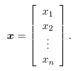
• A vector is an array of numbers. They are typically given lower-case variable names and are written in bold. An element of a vector (a scalar) is identified by writing its name in an italic typeface with a subscript.

• Sometimes, we need to index a set of elements of a vector. In this case, we define a set S containing the indices and write the set as a subset. The - sign is used to denote the complement of a set.

• Eg. S = {1, 3, 6} and $\boldsymbol{x}_S$

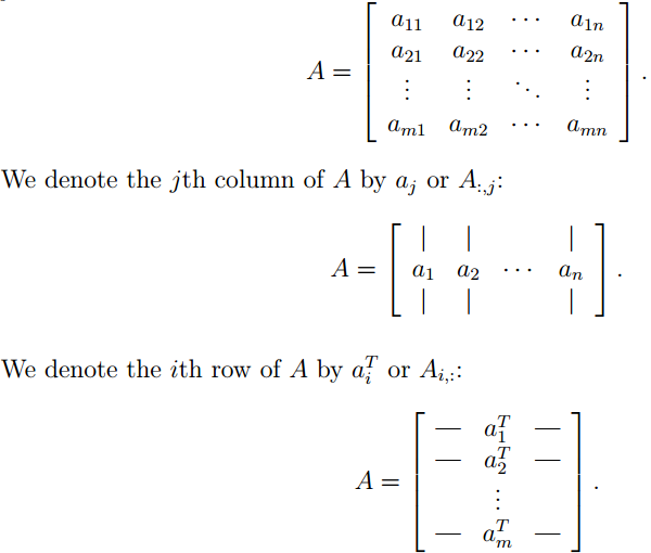
• A matrix is a 2-D array of numbers with each number identified by two indices instead of just one. They are usually given upper-case variable names with a bold typeface.

• Eg. $\boldsymbol{A}$

• An element of the matrix is referred to by using its name in italics, but not in bold. Eg. The upper left-most entry could be referred to using $\boldsymbol{A}_{1,1}$ The transpose of a matrix can be thought of as a mirror image across the main diagonal.

• $f\left( \boldsymbol{A} \right )_{i, j}$ gives the element (i, j) of the matrix computed by applying the function f to A.

• Tensors are arrays with more than two axes. They are usually represented by a bold typeface.

• Below is Python code to learn how to define and index scalars, vectors and matrices. The “shape” of an ndarray (numpy array) is its shape along each dimension, and is a very useful debugging tool. Note: These only cover the basics, and you can learn about advanced indexing here.

import numpy as np

# Define a scalar
s = 1
assert np.shape(s) == ()

# define a column vector
x = np.array([0, 1, 2])
assert x.shape == (3, )

# ndarray operations are defined element-wise by default
x_python_list = [0, 1, 2]
assert x_python_list * 2 == [0, 1, 2, 0, 1, 2]
assert np.array_equal(x*2, [0, 2, 4])
s = [0, 2] # set of indices whose values are to be retrieved
assert np.array_equal(x[s], [0, 2])

"""
np.arange can be used to create a sequence
np.reshape can be used to morph an array into a given shape
"""

# define a 3x3 matrix
A = np.arange(0, 9).reshape(3, 3)
assert A.shape == (3, 3)
assert A[0, 0] == 0
assert np.array_equal(A[0], [0, 1, 2]) # get row 0
assert np.array_equal(A[:, 0], [0, 3, 6]) # get column 0 

"""
Slicing basics -
Slicing uses the : operator whereas indexing does not
Slicing follows the convention; start:end:step - slicing three-tuple (i, j, k)
i.e. retrieve elements from the start index to end index jumping in steps=step
Default values:
 i = 0
 j = n if k > 0
 -1 if k < 0
 k = 1
Note that :: is the same as : and means select all indices along this axis.

For each dimension in the array, we can give i:j:k separated by a , 

Note: -ve index for start or end is interpreted as len(dimension) + index
 -ve index for step is interpreted as moving from larger to smaller index

A[0] is indexing row 0
A[0:] is slicing from row 0
A[:, 0] == A[0:3:1, 0] i.e. slice all rows and index 0th column

Note: Modifying a slice modifies the original array

"""

Multiplying Matrices and Vectors

An easy way to remember matrix multiplication is by looking at the dimensions of the matrices.

Vector-Vector Products

Given two vectors $x, y \in \mathbb{R}^{n}$

Inner Product (Dot Product)

Outer Product

Matrix-Vector Products

There are two ways to look at Matrix-Vector products. The first way is when the Matrix is on the left and the vector is on the right, and the second is when the Matrix is on the right and the vector is on the left. Consider a matrix $\boldsymbol{A} \in \mathbb{R}^{m \times n}$ and a vector $x \in \mathbb{R}^n$

Case 1: $y = \boldsymbol{A}x \in \mathbb{R}^m$

• Let us write A by rows. Then we find that the ith entry of $y$ is equal to the inner product of the ith row of $\boldsymbol{A}$ and $x$, i.e. $y_i = a_{i}^Tx$

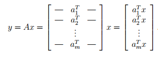
• Let us write A by columns. Then we can see that y is a linear combination of the columns of A where the coefficients of the linear combination are given by the entries of x.

Case 2: $y^T = x^T \boldsymbol{A}$

• If we express A by columns, the i^th entry of $y^T$ is equal to the inner product of $x$ and the i^th column of $\boldsymbol{A}$

• If we express A by rows, we see that $y^T$ is a linear combination of the rows of A where the coefficients of the linear combination are given by the entries of x .

Matrix-Matrix Products

Case 1: Matrix-Matrix multiplication viewed in the terms of Vector-Vector products.

• If we view A in rows and B in columns, the (i, j)^th entry of C is equal to the inner product of i^th row of A and the j^th column of B .

• If we view A in columns and B in rows, C is the sum of all outer products formed by the i^th column of A and the i^th row of B.

Case 2: Matrix-Matrix multiplication viewed in the terms of Matrix-Vector products.

• If we represent A as the matrix, and B by columns, the i^th column of C is given by Case-2 of Matrix-Vector products, i.e. vector on the right. c_i = A b_i .

• If we represent A in rows and B as the matrix, the ith row of C is given by Case-1 of Matrix-Vector products, i.e. vector on the left. c_i^T = a_i^T B .

• Some useful properties of Matrix multiplication

  • It is associative: (AB)C = A(BC).

  • It is is distributive: A(B + C) = AB + AC.

  • It is not commutative; AB $\neq$ BA.

Linear Dependence and Span

For a given system of equations Ax = b, it is possible to have exactly one solution, no solution or infinitely many solutions for some values of b. It is not possible, however, to have more than one but less than infinitely many solutions for a particular b. If we assume that x and y are solutions, then z = α x + (1 − α) y is also a solution for any real α.

The linear combination of a set of vectors is given by multiplying (scaling) each vector with a scalar, and then adding the result. The span of a set of vectors is the set of ALL points obtained by linear combination of the original vectors.

Each column of A can be looked at as a direction from the origin (vector of zeros), and x is the amount to travel in that direction. Determining whether Ax= b has a solution amounts to testing whether b is in the span of the columns of A (known as range or column space of A.)

If b is m-dimensional, then there need to be at least m columns in A, to move in m-directions to reach b from the origin. If this is not the case, there will be some values for b that can’t be reached using the directions of A, and the equation might have no solution. However, even if it has m-columns, if two columns are identical in their direction, one of them would be redundant. Formally, this redundancy is known as linear dependence . A set of vectors is linearly independent if no vector in the set is a linear combination of the others.

To ensure that there’s only one solution for b, we must ensure that A has at most m columns, otherwise there is more than one way of parameterizing each solution. Hence, to use the matrix inversion method, A must be a nonsingular square matrix.

The column/row rank of a matrix A_{m x n} is the largest number of columns/rows respectively of A that constitute a linearly independent set. It turns out that for any matrix, column rank = row rank, and are collectively referred to as the rank of A.

import numpy as np
from numpy.linalg import matrix_rank

I = np.eye(4)
assert matrix_rank(I) == 4 # Full rank identity matrix

I[-1,-1] = 0. # Create a rank deficient matrix
assert matrix_rank(I) == 3

O = np.ones((4,))
assert matrix_rank(O) == 1 # 1 dimension - rank 1 since all vectors are the same

O = np.zeros((4,))
assert matrix_rank(O) == 0 # Vectors don’t go in any direction

Norms

The size of the vector is usually measured by a function called norm. Formally, the $L^{p}$ is given as :

Norms are functions mapping vectors to nonnegative values. Intuitively norm measures the distance of the point from the origin. More rigorously, norm is a function which satisfies the following properties

The $L^2$ norm is called the Euclidean norm. It is used so frequently that the subscript p is dropped. It is also common to measure which is simple

Special Kinds of Matrices and Vectors

1. A diagonal matrix has entries only along the main diagonal. In D, D_i,j = 0 if i $\neq$ j. We can write diag( v ) to denote a square D whose diagonal entries are given by v . To compute diag( v ) x , we only need to scale each element x_i by v_i, i.e. diag( v )( x ) = v $\odot$ x . The inverse of D exists if every diagonal entry is nonzero, and diag( v ) -1 = diag ([1/v₁, … , 1/v_n]^T ). We may derive a very general ML algorithm in terms of arbitrary matrices, but obtain a less expensive (and less descriptive) algorithm by restricting some matrices to be diagonal. Non square diagonal matrices can be multiplied cheaply after concatenating zeroes to the result if D is taller than wide or discarding some of the last elements if D is wider than tall.

2. A symmetric matrix is one that is equal to its own transpose, i.e. A = A ^T. An antisymmetric is one where A = - A ^T. A + A ^T is symmetric and A - A ^T is antisymmetric. Thus, every square matrix can be represented as a sum of a symmetric and an antisymmetric matrix; A = 0.5 * (A + A ^T) + 0.5 * (A - A ^T).

3. A unit vector is a vector with unit norm, i.e. $\| x \|_2 = 1$

4. A vector x and a vector y are orthogonal to each other if x ^T y = 0. If two vectors are orthogonal and have unit norm, they are orthonormal. An orthogonal matrix is a square matrix whose rows are mutually orthonormal, and whose columns are mutually orthonormal, i.e. A ^T A = AA ^T = I, implying A ^-1 = A ^T. Note that operating on a vector with an orthogonal matrix will not change its Euclidean norm.

import numpy as np
import scipy

D = np.diag([1, 2, 4]) # Create a diagonal matrix

D_I = np.linalg.inv(D) # Find inverse of D

# Calculate the inverse based on diagonal property
diagonal = np.diag(D)
assert np.array_equal(D_I, np.diag(1.0 / diagonal))

"""
Create a symmetric matrix.
Fill A[i][j] and autofill a[j][i]
"""
A = np.zeros((3, 3))
A[0][1] = 1
A[1][2] = 2
A = A + A.T - np.diag(A.diagonal())
assert np.all(A == A.T) # Check for symmetric

# Some methods to create an orthogonal matrix
R = np.random.rand(3, 3)
Q = scipy.linalg.orth(R)
Q = scipy.stats.ortho_group.rvs(dim=3)
Q, _ = np.linalg.qr(R)

Eigen decomposition

An eigenvector of a square matrix A is a non-zero vector v such that multiplication by A alters only the scale of v : Av = λ v . Here, the scalar λ is the eigenvalue corresponding to the eigenvector v (Note: We can also find the left eigenvector such that v ^T A = λ v ^T ) If v is an eigenvector, then so is any rescaled vector sv (if s $\in \mathbb{R}, s > 0)$ with the same eigenvalue.

Suppose that a matrix A has n linearly independent eigenvectors, {v ⁽¹⁾, . . . ,v ⁽ⁿ⁾}, with corresponding eigenvalues {λ₁, . . . , λ_n}. We may concatenate all of the eigenvectors to form a matrix V with one eigenvector per column. Likewise, we can concatenate the eigenvalues to form a vector λ .

• The eigendecomposition of A is then given by A = V diag( λ ) V ⁻¹.

• Not every matrix can be decomposed into eigenvalues and eigenvectors. In some cases, the decomposition exists, but may involve complex rather than real numbers.

• Every real symmetric matrix can be decomposed into an expression using only real-valued eigenvectors and eigenvalues: A = Q 𝜦 Q ^T Where Q is an orthogonal matrix composed of eigenvectors of A, 𝜦 is a diagonal matrix,
  Eigenvalue 𝛬_i,i is associated with the eigenvector in column i of Q. Because Q is an orthogonal matrix, we can think of A as scaling space by λ_i in direction v⁽ⁱ⁾.

• Eigendecomposition may not be unique. If any two or more eigenvectors share the same eigenvalue, then any set of orthogonal vectors lying in their span are also eigenvectors with that eigenvalue, and we could equivalently choose a Q using those eigenvectors instead. By convention, we usually sort the entries of Λ in descending order. Under this convention, the eigendecomposition is unique only if all of the eigenvalues are unique.

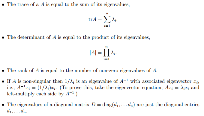
• A matrix whose eigenvalues are all positive is called positive definite. A matrix whose eigenvalues are all positive or zero-valued is called positive semidefinite. Likewise, if all eigenvalues are negative, the matrix is negative definite, and if all eigenvalues are negative or zero-valued, it is negative semidefinite. Positive semidefinite matrices are interesting because they guarantee that ∀ x , x ^T Ax ≥ 0.Positive definite matrices additionally guarantee that x ^T Ax = 0 ⇒ x = 0

• Note that only the symmetric part of A contributes to the quadratic form and so we often implicitly assume that the matrices appearing in a quadratic form are symmetric.

• One important property of positive definite and negative definite matrices is that they are always full rank, and hence, invertible.

• Given any matrix A ∈ R_m×n (not necessarily symmetric or even square), the matrix G = A ^T A (sometimes called a Gram matrix) is always positive semidefinite. Further, if m ≥ n (and we assume for convenience that A is full rank), then G = A ^T A is positive definite.

• An application where eigenvalues and eigenvectors come up frequently is in maximizing some function of a matrix max x ∈ R_n x ^T Ax subject to $\| x \|_{2}^2$ = 1. Assuming the eigenvalues are ordered as λ₁ ≥ λ₂ ≥ . . . ≥ λ_n, the optimal x for this optimization problem is x₁, the eigenvector corresponding to λ₁. We can also solve the minimization problem in the same way.

The following NumPy functions can be used for eigenvalue decomposition.

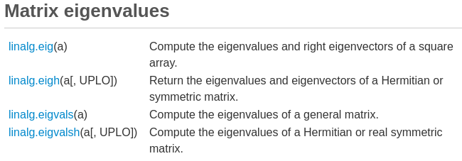
Please note that SciPy also has a linalg package. If possible, it is preferable to use the SciPy linalg package (after installing an optimized version of SciPy, because NumPy was built to be portable rather than fast and cannot use a FORTRAN compiler. SciPy on the other hand has access to the FORTRAN compiler and many lower level routines, and hence is preferred.)

Singular Value Decomposition

The previous section demonstrated decomposition of a matrix into eigenvalues and eigenvectors, however eigen decomposition is not generally applicable as a non-square matrix does not have an eigen decomposition. Another way to decompose a matrix is to factorize into singular values and singular vectors and this is called Singular Value Decomposition and is applicable for any real matrix. SVD is similar, except is defined as:

Suppose that A is an m x n matrix. Then U is defined to be an m x m matrix, D an m x n matrix, and V to be an n x n matrix.

U : Orthogonal matrix, columns are known as left-singular vectors and are the eigenvectors of AA ^T

V : Orthogonal matrix, columns are known as right-singular vectors and are the eigenvectors of A ^T A

D : Diagonal matrix, elements along the diagonal are known as singular values and are the non-zero singular values are the square roots of eigenvectors of AA ^T or A ^T A

SVD is useful as it allows us to partially generalize matrix inversion to non-square matrices.

import numpy as np
"""
    np.linalg.svd can be used to find the SVD for A
    It factorizes the matrix A as U * np.diag(d) * V
"""
A = np.random.rand(4, 3)  # Create a random matrix
U, d, V = np.linalg.svd(A)  # Finds the SVD for matrix A
D = np.zeros((4, 3))
D[:3, :3] = np.diag(d)  # Slice and assign the diagonal
assert U.shape == (4, 4)
assert V.shape == (3, 3)
assert np.allclose(A, np.dot(U, np.dot(D, V)))  #Reconstruct the matrix and compare

Moore-Penrose Pseudoinverse

Matrix inversion is not defined for non-square matrices. Recall the linear equation

If A is taller than it is wide, then it is possible for this equation to have no solution. If A is wider than it is tall, there could be multiple possible solutions. The pseudoinverse is defined as :

Practical definitions for computing pseudoinverse are not based on this formula, but are derived from the SVD. Hence, we can define the pseudoinverse A⁺ as :

Where U, D, V are the singular value decomposition of A. Note that the pseudoinverse of D is obtained by taking the reciprocal of its non-zero elements and then taking the transpose of the resulting matrix.

If A has more columns than rows (wider than tall), the pseudo inverse provides one of the many solutions, specifically it provides the solution with the minimum Euclidean norm.

$x = A^{+}y$ where x is the solution with the minimal Euclidean norm $\| x \|_2$

If A has more rows than columns (taller than wide), it is possible for there to be no solution. In this case, the solution x obtained minimizes the Euclidean norm $\| Ax - y \|_2$

import numpy as np

A = np.random.rand(3, 3)
B = np.linalg.pinv(A)
assert np.allclose(A, np.dot(A, np.dot(B, A))) # BA should be close to an identity matrix

Trace

The trace operator gives the sum of all the diagonal entries of a matrix:

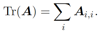
Trace operator allows us to conveniently specify certain operations. For example, the Frobenius norm can be elegantly defined as :

Some properties of the trace operator:

• Invariant to transpose : $Tr(\boldsymbol{A}) = Tr(\boldsymbol{A}^{T})$

• Scalar has its own trace $Tr(a) = a$

• Invariance to cyclic permutation : $Tr(\boldsymbol{A B C}) = Tr(\boldsymbol{C A B}) = Tr(\boldsymbol{B C A})$. This holds true even when the shape of the matrices are different. More generally,

import numpy as np
from math import sqrt

A = np.arange(9).reshape(3, 3)
assert np.trace(A) == 12

norm = np.linalg.norm(A)                     # Compute Frobenius norm
assert sqrt(np.trace(A.dot(A.T))) == norm    # Compare with the result from trace operator

Determinant

Determinant maps a matrix to a real valued scalar. Determinant is equal to the product of all the eigenvalues of the matrix. It can be thought of how much multiplication by the matrix expands or contracts space. If determinant is 0, the matrix loses all of its volume and is contracted completely across at least one dimension. If determinant is 1, then the transformation preserves volume. Determinant is denoted as $det(\boldsymbol{A})$

import numpy as np


A = np.array([[1, 2], [3, 4]])
print np.linalg.det(A)

Matrix Calculus

Coming soon!

References

[1] http://www.deeplearningbook.org/contents/linear_algebra.html

[2] http://cs229.stanford.edu/section/cs229-linalg.pdf

[3] http://cs231n.github.io/python-numpy-tutorial/

[4] http://www.bogotobogo.com/python/python_numpy_array_tutorial_basic_A.php

[5] http://www.bogotobogo.com/python/python_numpy_array_tutorial_basic_B.php

[6] http://www.bogotobogo.com/python/python_numpy_matrix_tutorial.php